One of the main objectives of research Research Critical and exhaustive investigation or experimentation, having for its aim the discovery of new facts and their correct interpretation, the revision of accepted conclusions, theories, or laws in the light of newly discovered facts, or the practical application of such new or revised conclusions, theories, or laws. Conflict of Interest and medical studies is to learn what associations or outcomes are not a product Product A molecule created by the enzymatic reaction. Basics of Enzymes of chance. According to the study's design and the data it provides, a hypothesis can be accepted or rejected, allowing for a determination in correlation Correlation Determination of whether or not two variables are correlated. This means to study whether an increase or decrease in one variable corresponds to an increase or decrease in the other variable. Causality, Validity, and Reliability. Statistical tests are tools used by researchers to obtain information and meaning from pools of variable Variable Variables represent information about something that can change. The design of the measurement scales, or of the methods for obtaining information, will determine the data gathered and the characteristics of that data. As a result, a variable can be qualitative or quantitative, and may be further classified into subgroups. Types of Variables data. These tests come in several forms, including, for example, the chi-square and Fisher exact tests, and are chosen depending on the needs of the investigators and the characteristics of the variables being analyzed. Study results can be considered statistically significant based on calculated p-values and predetermined levels of significance (known as the α-level). Confidence intervals are another way to express the significance of a statistical result without using a p-value.
Last updated: Dec 15, 2025
Hypothesis testing is used to assess the plausibility of a hypothesis by analyzing study data.
For example, a company creates a new Drug X that is intended to treat hypertension Hypertension Hypertension, or high blood pressure, is a common disease that manifests as elevated systemic arterial pressures. Hypertension is most often asymptomatic and is found incidentally as part of a routine physical examination or during triage for an unrelated medical encounter. Hypertension. The company wants to know whether Drug X does in fact work to lower BP, so they need to do hypothesis testing.
Steps for testing a hypothesis:
A hypothesis is a preliminary answer to a research Research Critical and exhaustive investigation or experimentation, having for its aim the discovery of new facts and their correct interpretation, the revision of accepted conclusions, theories, or laws in the light of newly discovered facts, or the practical application of such new or revised conclusions, theories, or laws. Conflict of Interest question (i.e., a “guess” about what the results will be). There are 2 types of hypotheses: the null hypothesis and the alternative hypothesis.
Example 1: rejecting the null hypothesis
In the example above, if the findings of the trial show that Drug X does in fact significantly lower BP (that is, there is sufficient statistical evidence to support it), then the null hypothesis (postulating that there is no difference between the groups) is rejected with a given probability Probability Probability is a mathematical tool used to study randomness and provide predictions about the likelihood of something happening. There are several basic rules of probability that can be used to help determine the probability of multiple events happening together, separately, or sequentially. Basics of Probability. Note that these findings cannot confirm the alternative hypothesis, but only support it with a given probability Probability Probability is a mathematical tool used to study randomness and provide predictions about the likelihood of something happening. There are several basic rules of probability that can be used to help determine the probability of multiple events happening together, separately, or sequentially. Basics of Probability, determined by the sampling distribution in the population tested.
Example 2: failing to reject the null hypothesis
In the example above, if the findings of the trial show that Drug X did not significantly lower BP, then the study failed to reject the null hypothesis. Again, note that the findings cannot confirm the null hypothesis but only support it with a given probability Probability Probability is a mathematical tool used to study randomness and provide predictions about the likelihood of something happening. There are several basic rules of probability that can be used to help determine the probability of multiple events happening together, separately, or sequentially. Basics of Probability, determined by the sampling distribution in the population tested.

Types of errors
Image by Lecturio.Statistical significance is the idea that all test outcomes are highly unlikely to be produced simply by chance. To determine statistical significance, you need to set an α-value and calculate a p-value.
A graph can be created in which possible study results are plotted on the x-axis and the probability Probability Probability is a mathematical tool used to study randomness and provide predictions about the likelihood of something happening. There are several basic rules of probability that can be used to help determine the probability of multiple events happening together, separately, or sequentially. Basics of Probability of observing each result are plotted on the y-axis. The area under the curve represents the p-value.
Mnemonic:
“If the p is low, the null (hypothesis) must go.”
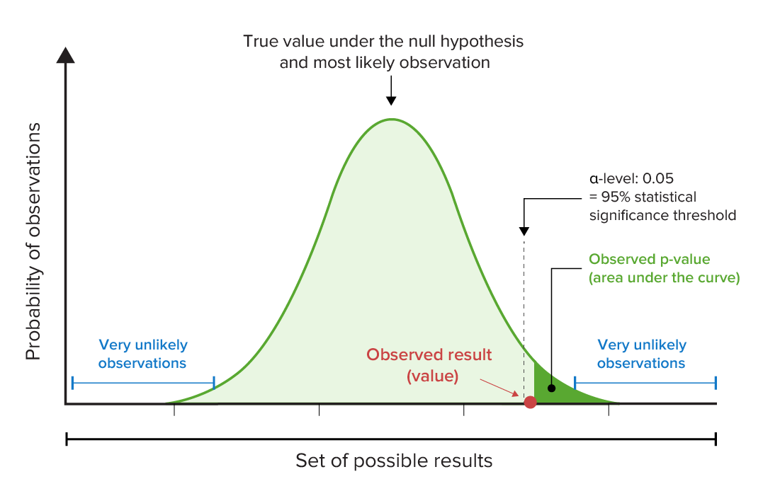
Graphical representation of the p-value and α-levels:
Note, in this example, that the observed p-value is less than the predetermined level of statistical significance (in this case, 95%). This means that the null hypothesis should be rejected because the observed result would be very unlikely if the null hypothesis (that no relationship exists between variables) were true.
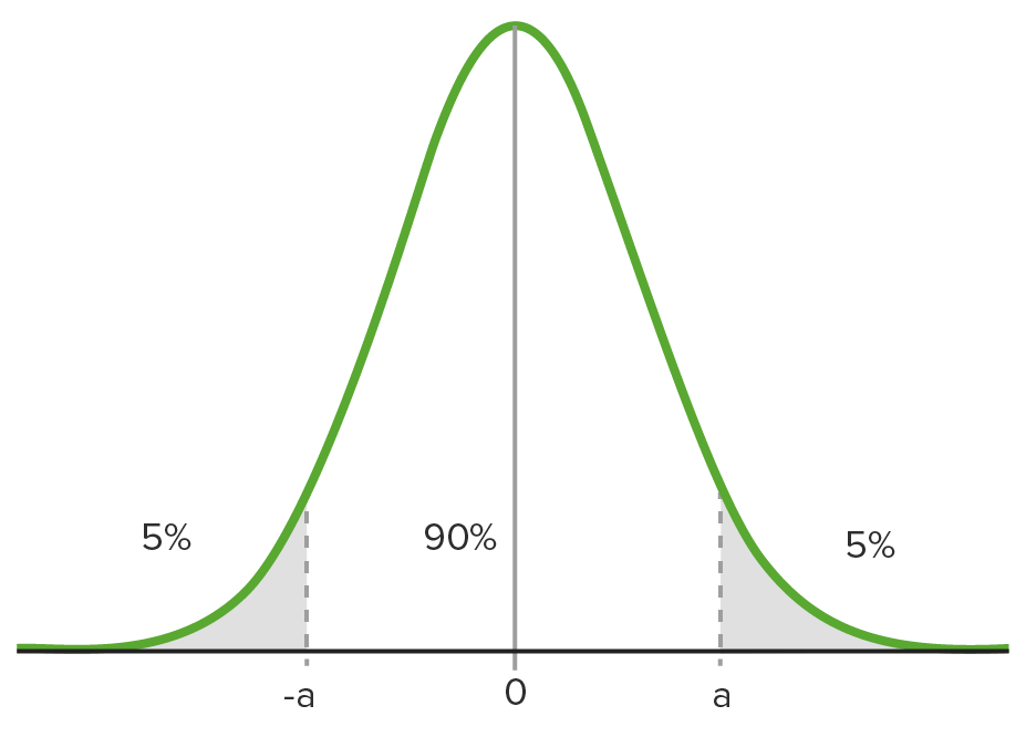
A 90% confidence interval on a standard normal curve
Image by Lecturio.Your choice of test is based on:
The reasonability of the model should always be questioned. If the model is wrong, so is everything else.
Be careful of variables that are not truly independent.
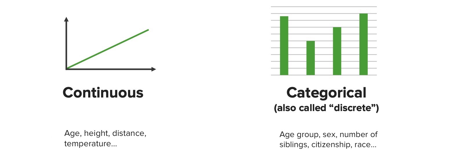
Graphical representations of continuous and categorical data
Image by Lecturio. License: CC BY-NC-SA 4.0The 3 primary categories of statistical tests are:
| Test name | What the test is testing | Types of variables/data | Example |
|---|---|---|---|
| Regression Regression Corneal Abrasions, Erosion, and Ulcers tests | |||
| Simple linear regression Regression Corneal Abrasions, Erosion, and Ulcers | How a change in the predictor/input variable Variable Variables represent information about something that can change. The design of the measurement scales, or of the methods for obtaining information, will determine the data gathered and the characteristics of that data. As a result, a variable can be qualitative or quantitative, and may be further classified into subgroups. Types of Variables affects the outcome variable Variable Variables represent information about something that can change. The design of the measurement scales, or of the methods for obtaining information, will determine the data gathered and the characteristics of that data. As a result, a variable can be qualitative or quantitative, and may be further classified into subgroups. Types of Variables |
|
How does weight (predictor) affect Affect The feeling-tone accompaniment of an idea or mental representation. It is the most direct psychic derivative of instinct and the psychic representative of the various bodily changes by means of which instincts manifest themselves. Psychiatric Assessment life expectancy Life expectancy Based on known statistical data, the number of years which any person of a given age may reasonably expected to live. Population Pyramids (outcome)? |
| Multiple linear regression Regression Corneal Abrasions, Erosion, and Ulcers | How changes in the combinations of ≥ 2 predictor variables can predict changes in the outcome |
|
How do weight and socioeconomic status (predictors) affect Affect The feeling-tone accompaniment of an idea or mental representation. It is the most direct psychic derivative of instinct and the psychic representative of the various bodily changes by means of which instincts manifest themselves. Psychiatric Assessment life expectancy Life expectancy Based on known statistical data, the number of years which any person of a given age may reasonably expected to live. Population Pyramids (outcome)? |
| Logistic regression Regression Corneal Abrasions, Erosion, and Ulcers | How ≥ 1 predictor variables can affect Affect The feeling-tone accompaniment of an idea or mental representation. It is the most direct psychic derivative of instinct and the psychic representative of the various bodily changes by means of which instincts manifest themselves. Psychiatric Assessment a binary outcome |
|
What is the effect of weight (predictor) on survival (binary outcome: dead or alive)? |
| Comparison tests | |||
| Paired t-test T-test Statistical Power | Compares the means of 2 groups from the same population |
|
Compare the weights of infants (outcome) before and after feeding (predictor). |
| Independent t-test T-test Statistical Power | Compares the means of 2 groups from different populations |
|
What is the difference in average height (outcome) between 2 different basketball teams (predictor)? |
| Analysis of variance (ANOVA) | Compares the means from > 2 groups |
|
What is the difference in blood glucose Glucose A primary source of energy for living organisms. It is naturally occurring and is found in fruits and other parts of plants in its free state. It is used therapeutically in fluid and nutrient replacement. Lactose Intolerance levels (outcome) 1, 2, and 3 hours after a meal (predictors)? |
| Correlation Correlation Determination of whether or not two variables are correlated. This means to study whether an increase or decrease in one variable corresponds to an increase or decrease in the other variable. Causality, Validity, and Reliability tests | |||
| Chi-square test | Tests the strength of association between 2 categorical variables with a larger sample size Sample size The number of units (persons, animals, patients, specified circumstances, etc.) in a population to be studied. The sample size should be big enough to have a high likelihood of detecting a true difference between two groups. Statistical Power |
|
Compare whether acceptance into medical school ( variable Variable Variables represent information about something that can change. The design of the measurement scales, or of the methods for obtaining information, will determine the data gathered and the characteristics of that data. As a result, a variable can be qualitative or quantitative, and may be further classified into subgroups. Types of Variables 1) is more likely if the applicant was born in the United Kingdom ( variable Variable Variables represent information about something that can change. The design of the measurement scales, or of the methods for obtaining information, will determine the data gathered and the characteristics of that data. As a result, a variable can be qualitative or quantitative, and may be further classified into subgroups. Types of Variables 2). |
| Fisher’s exact test | Tests the strength of association between 2 categorical variables with a smaller sample size Sample size The number of units (persons, animals, patients, specified circumstances, etc.) in a population to be studied. The sample size should be big enough to have a high likelihood of detecting a true difference between two groups. Statistical Power |
|
Same as chi-square, but with smaller sample sizes |
| Pearson r test | Tests the strength of association between 2 continuous variables |
|
Compare how plasma Plasma The residual portion of blood that is left after removal of blood cells by centrifugation without prior blood coagulation. Transfusion Products HbA1c level ( variable Variable Variables represent information about something that can change. The design of the measurement scales, or of the methods for obtaining information, will determine the data gathered and the characteristics of that data. As a result, a variable can be qualitative or quantitative, and may be further classified into subgroups. Types of Variables 1) is related to plasma Plasma The residual portion of blood that is left after removal of blood cells by centrifugation without prior blood coagulation. Transfusion Products triglyceride levels ( variable Variable Variables represent information about something that can change. The design of the measurement scales, or of the methods for obtaining information, will determine the data gathered and the characteristics of that data. As a result, a variable can be qualitative or quantitative, and may be further classified into subgroups. Types of Variables 2) in diabetic patients Patients Individuals participating in the health care system for the purpose of receiving therapeutic, diagnostic, or preventive procedures. Clinician–Patient Relationship. |
Chi-square tests are commonly used to analyze categorical data and determine whether 2 categorical variables are related.
In order to perform a chi-square test, 2 pieces of information are needed: the degrees of freedom (number of categories minus 1), and the α-level (which is chosen by the researcher and usually set at 0.05). In addition, the data should be organized in a table.
Example: If you wanted to see whether jugglers were more likely to be born during a particular season, the data could be recorded in the following table:
| Category (i): season of birth | Observed frequency of jugglers in each birth season |
|---|---|
| Spring | 66 |
| Summer | 82 |
| Fall | 74 |
| Winter Winter Pityriasis Rosea | 78 |
To begin, the expected frequencies for each cell in the table above need to be determined using the equation:
$$ Expected\ frequency = np_{0i} $$where n = the sample size Sample size The number of units (persons, animals, patients, specified circumstances, etc.) in a population to be studied. The sample size should be big enough to have a high likelihood of detecting a true difference between two groups. Statistical Power and p0i is the hypothesized proportion in each category i.
In the above example, n = 300 and p0i is ¼, so the expected cell frequency is 300 * 0.25 = 75 in each cell.
The test statistic is then calculated by the standard chi-square formula:
$$ \chi ^{2} = \sum _{all\ cells} \frac{(observed-expected)^{2}}{expected} $$where 𝝌2 is the test statistic being calculated. For each “cell” or category, the expected frequency is subtracted from the observed frequency; this value is squared and then divided by the expected frequency. After this number is calculated for each category, the numbers are added together.
Example 𝝌2 calculation: Using the example above, the expected frequency in each cell is 75, so the 𝝌2 test statistic can be calculated as follows:
| Category (i): season of birth | Observed frequency of jugglers with each birth season | (Observed – expected)2/expected |
|---|---|---|
| Spring | 66 | (66 ‒ 75)2 / 75 = 1.08 |
| Summer | 82 | (82 ‒ 75)2 / 75 = 0.653 |
| Fall | 74 | (74 ‒ 75)2 / 75 = 0.013 |
| Winter Winter Pityriasis Rosea | 78 | (78 ‒ 75)2 / 75 = 0.12 |
𝝌2 = 1.08 + 0.653 + 0.013 + 0.12 = 1.866
Determining whether or not the test statistic is statistically significant:
To determine whether this test statistic is statistically significant, the chi-square table is used to obtain the chi-square critical number.
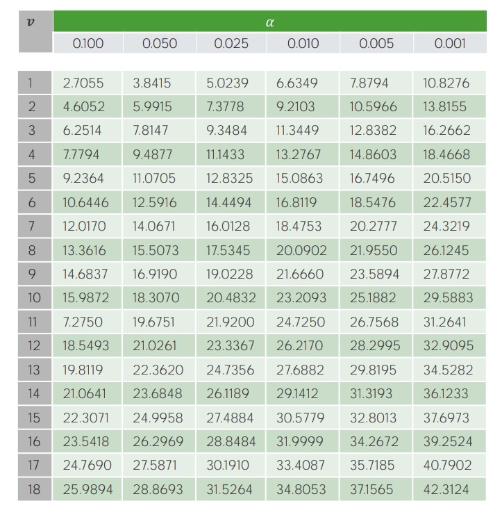
Example of the critical value table for the 𝝌2 test:
On the y-axis, V represents the degrees of freedom (i.e., the number of categories being studied minus 1); significance levels (α-levels) are shown along the x-axis. The corresponding critical values are found in the table and then compared to the calculated test statistic.
Example 𝝌2 test: Are jugglers more likely to be born in a particular season at a 0.05 significance level?
| Category (i): season of birth | Observed frequency of jugglers with each birth season | (Observed ‒ expected)2/expected |
|---|---|---|
| Spring | 66 | (66 ‒ 75)2 / 75 = 1.08 |
| Summer | 82 | (82 ‒ 75)2 / 75 = 0.653 |
| Fall | 74 | (74 ‒ 75)2 / 75 = 0.013 |
| Winter Winter Pityriasis Rosea | 78 | (78 ‒ 75)2 / 75 = 0.12 |
𝝌2 = 1.08 + 0.653 + 0.013 + 0.12 = 1.866
Since 1.866 is < 7.81 (our critical value), we need to fail to reject (i.e., accept) the null hypothesis and conclude that season of birth is not associated with juggling.
Common pitfalls Pitfalls Basics of Probability:
Similar to the 𝝌2 test, the Fisher’s exact test is a statistical test used to determine whether there are nonrandom associations between 2 categorical variables.
A 2 × 2 contingency table Contingency table A contingency table lists the frequency distributions of variables from a study and is a convenient way to look at any relationships between variables. Measures of Risk is set up like this:
| Y | Z | Row total | |
|---|---|---|---|
| W | A | B | A + B |
| X | C | D | C + D |
| Column total | A + C | B + D | A + B + C + D (= n) |
The test statistic, p, is calculated from this table using the following formula:
$$ p = \frac{(\frac{a+b}{a})(\frac{c+d}{c})}{(\frac{n}{a+c})} = \frac{(\frac{a+b}{b})(\frac{c+d}{d})}{(\frac{n}{b+d})} = \frac{(a+b)! (c+d)! (a+c)! (b+d)!}{a! b! c! d! n!} $$where p = p-value; A, B, C, and D are numbers from the cells in a basic 2 × 2 contingency table Contingency table A contingency table lists the frequency distributions of variables from a study and is a convenient way to look at any relationships between variables. Measures of Risk; and n = total of A + B + C + D.
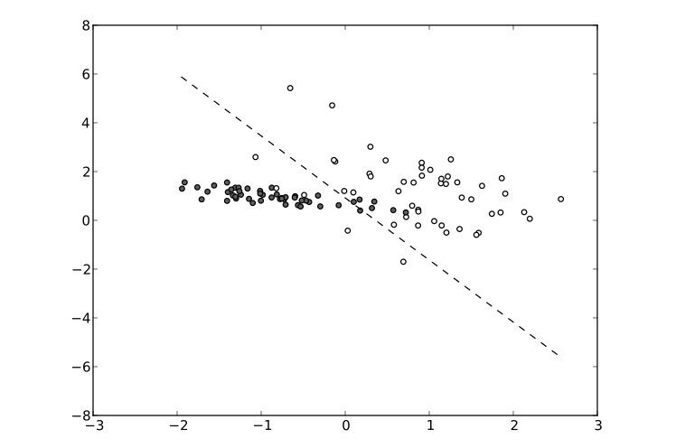
Before any calculations are made, data should be presented in a simple graphical format (e.g., bar graph, scatter plot, histogram Histogram Population Pyramids).
Contingency tables:
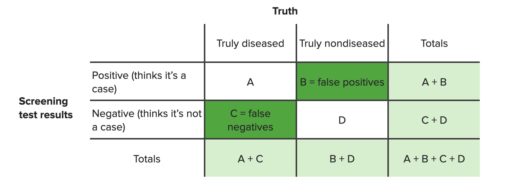
Contingency table identifying false positives (b) and false negatives (c)
Image by Lecturio. License: CC BY-NC-SA 4.0Scatter diagram or dispersion Dispersion Central tendency is a measure of values in a sample that identifies the different central points in the data, often referred to colloquially as “averages.” The most common measurements of central tendency are the mean, median, and mode. Identifying the central value allows other values to be compared to it, showing the spread or cluster of the sample, which is known as the dispersion or distribution. Measures of Central Tendency and Dispersion diagrams:
Box plots:
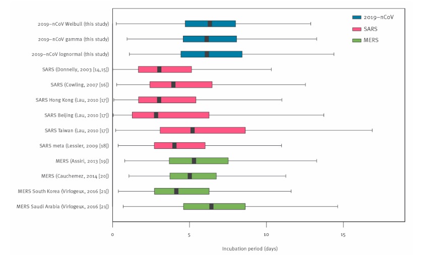
Example of a box plot
Image: “Box-and-whisker-plots” by Jantien A. Backer, Don Klinkenberg, Jacco Wallinga. License: CC BY 4.0Kaplan-Meier survival curves
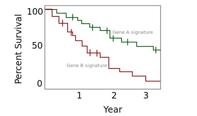
Example of a Kaplan-Meier plot
Image: “An example of a Kaplan Meier plot” by Rw251. License: CC0 1.0Tables (a frequency table is 1 example):
Histograms:
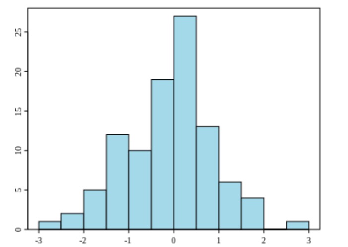
Example of a histogram
Image: “Example of a histogram” by Jkv. License: Public DomainFrequency polygon charts:
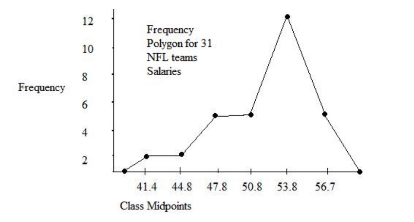
Frequency polygon chart for salaries of 31 NFL teams
Image: “Example of a frequency polygon chart” by JLW87. License: Public DomainFrequency tables, bar charts/histograms, and pie charts are 3 of the most common ways to present categorical data.
Frequency tables:
| Stoplight color | Frequency |
|---|---|
| Red | 65 |
| Yellow | 5 |
| Green | 30 |
Bar graph:
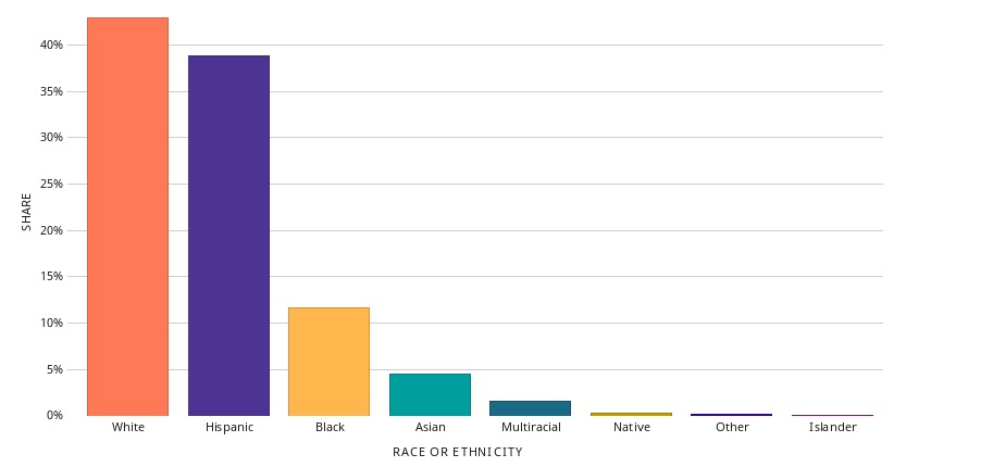
Example of a bar graph
Image: “Bar Chart of Race & Ethnicity in Texas” by Datawheel. License: CC0 1.0Pie charts:
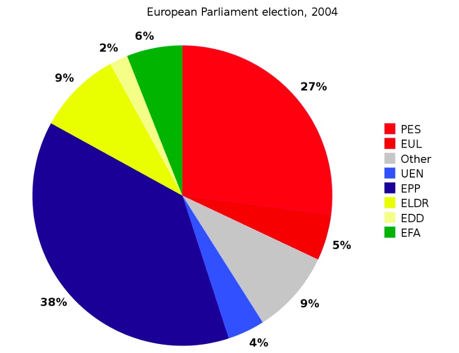
Example of a pie chart
Image: “A pie chart for the example data” by Liftarn. License: Public Domain