Playlist
Show Playlist
Hide Playlist
General Rules of Probability

-
Slides Statistics pt1 General Rules of Probability.pdf
-
Download Lecture Overview
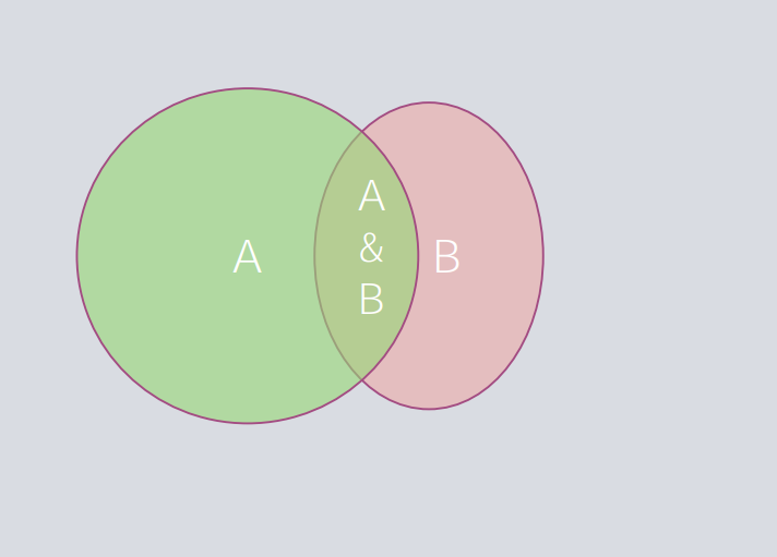
00:01 Welcome back for lecture 12, where we're gonna discuss more rules of probability. 00:05 Let's motivate what we're gonna do with an example. 00:08 Supposed we're in a bank and we're sorting out money. 00:11 We have several $1, $2, $5, $10, $20, $50 and $100, and we wanna draw a pile, a bill from this pile without looking at it. 00:20 The sample space is $1, $2, $5, $10, $20, $50 and $100. 00:27 We can make different events out of the sample space. 00:30 Suppose we let A be the event that we get a $1, $5 or a $10. 00:34 B could be the event that we get a bill without a president on it, just the $10 and the $100. 00:39 We could let C be the event that we have, that we draw enough to pay for a $12 meal with it so that would include, $20s, $50 and $100s. But let's look at the events more closely. 00:51 If we have 8 $1 bills, 4 $2 bills, 6 $5 bills, 4 $10 bills, 1 $20 bill, 2 $50 bills and 3 $100 bills, then drawing a $1 bill does not happen with the same probability as drawing say a $5 bill. 01:08 For instance, the probability of drawing a $10 bill, a $20 bill and a $50 bill is not 3/7 just because those are three different possible outcomes and there are 7 possible outcomes. 01:21 There are 7 types of bills but each of them are represented in different numbers from the others. 01:28 Let's go back to those, consider the events A which is drawing a bill with an odd-numbered value, and B the event that we draw a bill with a building on the back of it. 01:40 The event A is comprised of the denominations $1 and $5. 01:45 The event B is comprise of the denominations $5, $10, $20, $50 and $100. 01:51 Note that $5 bills are in both events, therefore these two events are not disjoint. 01:58 If we want the probability that A or B happens we cannot use the addition rule that we learned in lecture 11. 02:05 If we add the probability of A and the probability of B. 02:10 Then, what we have added is the probability of a $5, $10, $20, $50 or a $100 and the probability of a $1 or a $5. 02:17 What did we do? We counted the probability of a $5 bill two times. 02:22 Observe that the $5 bill is A intersect B, that's where A and B both happen at the same time. 02:31 In order to fix the problem of having counted the $5 bill twice. 02:35 We need to subtract off the probability of the $5 bill one time, which is the probability of A and B. 02:41 So that's how we fix that problem. 02:43 Let's look at the general addition rule, formerly stated and then in the picture. 02:48 In general, the probability of an event A occurring or B happening or both is the probability of A or B which is given by P of A plus P of B, minus the probability of A and B, and this is illustrated in the Venn diagram down below. 03:05 Where we have one circle corresponding to A, one circle corresponding to B and then the overlap region for A and B. 03:14 Now, remember again that the boxes, the sample space it has probability 1. 03:18 The probability of A corresponds to the probability in the circle corresponding to A, and the probability of B is represented by the probability in the circle corresponding to B. 03:28 When we overlap them, if we add the probability in the first circle to the probability in the second circle, we have that overlap area counted twice so we need to get rid of that once, and that's why we subtract the probability of A and B. 03:42 We want to find the probability that one or the other or both happen. 03:46 Let's look at contingency tables and their role in probability and we're gonna do this by example as well. 03:52 In this example we have two psychologists the survey 478 4th, 5th and 6th graders from several schools, and we ask them if their primary goal is to get good grades, to be popular or to be good at sports. 04:06 This is the contingency table of the results by sex of the child and their goals. 04:12 Here we go, here are all the numbers in the table and using this table we can answer several questions. 04:19 For example, we can answer the question of, what is the probability that a person selected at random from these students is a girl? There are 251 girls out of the 478 students. 04:34 The probability of a girl is 251 out of 478 or 0.525. 04:39 What is the probability that a randomly selected student aspires to excel in sports? We have 90 students out of the 478 that want to excel at sports. 04:50 The probability of wanting to excel at sports is 90 out of 478 or 0.188. 04:57 We can find other probabilities form the table What is the probability that a randomly selected student is a girl who hopes to excel at sports? What we're looking at is the probability -- we want the probability of a girl and aspiring to excel at sports. 05:12 We have 30 students that are girls that hope to excel at sports so the probability of both of these two things happening is 30 out of 478 or 0.063. 05:22 Other things we might wanna do. 05:25 We might wanna look at how boys and girls compare with respect to goals. 05:28 We found conditional -- we have before found conditional distributions using the contingency table, and we can apply similar techniques to find conditional probabilities. 05:38 Let's look at using the contingency table as a way to introduce ourselves to conditional probability. 05:45 If we wanna look at the probability for instance that a boy hopes to excel at sports. 05:51 We need only look at the boys. 05:53 If we wanna find the probability that the student wishes to excel at sports given that the student is a boy. 05:59 Let's find this probability and then find similar one for girls. 06:03 We have 251 girls and 30 of them hope to excel at sports. 06:09 We have 227 boys and 60 of them hope to excel at sports. 06:15 Therefore, the probability of hoping to excel at sports, given that a person is a girl is 30 out of the number of girls which is 251 or 0.12. 06:25 The probability of hoping to excel at sports given that student is a boy is 60 out of the number of boy which is 227. 06:33 We get 0.264 as a probability of hoping to excel at sports given that we found a boy. 06:39 Let's look at conditional probability a little bit closer. 06:43 The last two probabilities are examples of what we call conditional probabilities. 06:48 If we want the probability of an event from a conditional distribution, we write the probability of B given A, that's how this symbolization is written, P of B line A means the probability of P given A or the probability that B happens given that the event A has occurred. 07:06 Let's look again a probability of aspiring at sports given that we found a girl. 07:10 Since we are looking at the conditional distribution of goals among the girls, we just restrict our attention to the girls and count the students who are girls and they hoped to excel at sports. 07:22 This leads us to the formal definition of conditional probability. 07:26 The probability of B given A is given by the probability of A and B divided by the probability of A. 07:34 Let's go back and do it again using the rules of probability. 07:38 Let's find the probability of sports given the girl. 07:42 What we found before was that the probability of a girl is 251 out 478. 07:48 We found that the probability of sports and girl is 30 out of 478. 07:53 The probability of sports given the girl is the probability of sports and girl divided by the probability that the student is a girl so we get 30 out of 478 divided by 251 out of 478 which is 30 divided by 251. 08:10 This is P of A given B and note to that matches what we found before. 08:15 How can we tell if two events are independent? Or we say formally that two events A and B are independent if the probability of B given A is equal to the probability of B. 08:26 Without the math what that means is knowing that A occurs has no impact on the probability that B occurs. 08:34 The question now as an example is, are hoping to excel in sports and the students sex independent? Well, let's look at the answer to that question. We found that the probability of sports given girl is 0.12. 08:47 The probability of hoping to aspire at sports is 90 out of 478 or 0.188, these aren't the same. 08:56 The hope to excel in sports and sex are not independent. 09:02 Now we can examine tables, Venn diagrams and probability and how we displaying picture probabilities. 09:09 We do these things using tables and Venn diagrams and we’ve seen both of these at work before. 09:14 Contingency table gives us an easy way to think about conditional probabilities. 09:19 Often, we're given probabilities without a table. 09:22 We can still construct one given the information that we have. 09:25 Let's look at an example. 09:28 Police report that 76% or 78% of drivers stop for suspension of drink driving are given a breath test, 36% are given a blood test, and 22% are given both. 09:40 We can use this information to construct the table. 09:42 We’re given that the probability of a breath test and the blood test is 0.22. 09:48 The probability that the driver gets a blood test is 0.36 and the probability of a breath test is 0.78. 09:56 We can start by remembering our rules of probability and we can use them to construct the rest of the table. 10:01 In making the table, let's just fill in what we know. 10:04 We have the blood test on the left hand side, the breath test going across the top. 10:09 We know that the probability of a blood test is 0.36 and the probability of both a blood test and a breath test is 0.22, so we fill those in. 10:18 We also know that the probability of a breath test is 0.78. 10:23 Now, we have to fill in the rest. 10:25 What we know is that since the probability of a blood test is 0.36 and then of this 0.36, 0.22 also get a breath test, what we have left over is the probability of the blood test with no breath test is 0.36 minus 0.32 or 0.22 excuse me is 0.14. 10:46 We also know that the probability of a breath test is 0.78 and that the probability of both test is 0.22. 10:55 What this leaves leftover for the probability of a breath test and no blood test is 0.78 minus 0.22 or 0.56. 11:05 We know that all the probabilities in the table -- in the body of the table have to add up to 1. 11:10 So that gives us the last probability in the body of the table which is the probability of no blood test and no breath test. 11:17 We get 1 minus 0.14 minus 0.56 minus 0.22 gives us 0.08. 11:24 We can fill in the cells in the margins now too. 11:27 Probability of no breath test is equal to 1 minus the probability of a breath test or 1 minus 0.78 which is 0.22. 11:36 Probability of no blood test is 1 minus the probability of a blood test or 1 minus 0.36 which gives us 0.64. 11:45 Here's the table now, once we fill in everything. 11:48 From the three pieces of information we were given at the beginning of the question. 11:53 We were able to fill in all these other information in the table. 11:56 We can use the table to answer more questions. 12:00 The first is, are getting a blood test and a breath test disjoint? Well no, the probability of getting a blood test and a breath test is 0.22 which is 0. 12:11 These two things can occur together so blood test and breath test are not disjoints events. 12:16 Are getting a blood test and a breath test independent? No, probability of getting a blood test given that you got a breath test is probability of blood and breath divided by the probability of breath just 0.22 divided by 0.78 or 0.282. 12:34 The probability of a blood test is 0.36 which is not the same is that conditional probability we just found. 12:41 Blood test and breath test are not independent. 12:44 What do we do when two events are not independent? We know what we do when two events aren't disjoint. 12:51 Now, we have to figure out what we can do when two events are not independent. 12:54 Recall that if two events A and B are independent then the probability of A and B is just equal to the probability of A times the probability of B. 13:03 If they're not independent then we have another result. 13:07 Recall that the probability of A given B is equal to the probability of A and B divided by the probability of B. 13:14 Now, we just do some algebra. 13:16 In general, what we have is the probability of A and B is equal to the probability of A given B times the probability of B. 13:24 We call this the general multiplication rule. 13:27 If A and B are independent, remember that the probability of A given B is equal to the probability of A, so probability of A intersect B is equal to the probability of A times the probability of B. 13:40 The general multiplication rule, gives rise to the multiplication rule for independent events. 13:46 In the example, let's find the probability of blood intersect breath using the probabilities that we have available. 13:54 We know that the probability of blood giving breath is equal to 0.282. 14:00 We know that the probability of breath is 0.78. 14:04 We get the probability of blood and breath is 0.282 times 0.78 which is 0.22, this matches the result that we got in the table and the information that we were given in the beginning of the problem. 14:19 Let's look at the picture. Here is the breath test. 14:22 Let's look into center first. We have 0.22 in the middle. 14:26 We have in total probability of breath is 0.78 so that leaves 0.56 probability in breath circle without being in the overlap region. 14:37 And the blood test we have 0.36. 14:40 We have 0.22 in the overlap region, so that leaves 0.14 in the blood test region and then 0.08 left in the region that corresponds to no blood test and no breath test. 14:51 Sometimes we like to draw things without replacement. 14:55 We'll go back to the money example to illustrate this. 14:58 Suppose we just draw a bill and we get a $10 bill, and then we wanna draw another one. 15:04 What’s the probability that we draw another $10 bill. 15:07 What is the probability that we draw a $10 on the first draw and a $10 on the second draw is what we're asking. 15:13 We do not put the first bill back into the pile. 15:16 On the first draw, there are total of 28 bills available, 8 of these are $10 bills. 15:23 We have drawn -- if we have drawn a $10 on the first draw, what we're interested in is the probability of a $10 bill on the second given that we drew a $10 bill on the first. 15:34 So what happens? After the first draw, there are 27 bills remaining and of those remaining bills since we drew a $10 bill on the first one, 7 are $10 bills. 15:46 The probability of a $10 bill on a second given a $10 bill on the first is 7 out of 27. 15:53 What is the probability that we draw $10 bills on both draws? This is not the same as the question that we just answered. 16:02 What we were interested in now is the probability that we draw a $10 bill on the first draw, and we draw a $10 bill on the second draw. 16:09 This is not a conditional probability. 16:11 This isn't an probability, so we need to use the general multiplication rule. 16:15 The probability of a $10 on a first and a $10 on a second is the probability of a $10 on a second, given a $10 on the first times the probability of a $10 on the first. 16:25 On the first draw, there are 28 available bills, 8 of which are $10 bills so the probability of drawing a $10 bill on the first is 8 out of 28. 16:34 Therefore, the probability of a $10 on the first and the $10 on the second is 7 out of 27 times 8 out of 28 or 0.0741. 16:45 This idea of sampling without replacement gives rise to a more general way of using pictures to think about probability. 16:53 We're gonna look at what a Tree Diagram does. 16:56 It's another visual representation of probability. 16:59 Let's say that a recent survey in Maryland found that in 77% of all accidents, the driver was wearing a seat belt. 17:06 92% of those drivers escaped serious injury and only 63% of the non-belted drivers were able to not be seriously injured. 17:16 We can make a tree diagram for this information. 17:19 It makes it easier to employ the general multiplication rule because we can separate and find the probabilities and write them out as a picture. 17:27 For this example, let's first spearate the drivers by whether or not they wear a seatbelt. 17:32 The separation is pictured down here in this beginning of a tree diagram. 17:36 We have the probability of wearing a seatbelt, 77% or 0.77, no seatbelt, 0.23. 17:45 In the second level of a tree, now we can put in the conditional probabilities. 17:50 We're given in the statement of the problem that of the people who wear seatbelts, 92% of them were okay, so that means that the probability that someone is okay in an accident given that they were wearing their seatbelt is 0.92. 18:05 So that means that the probability that somebody was injured given that they were wearing their seatbelt is 0.08. 18:10 If they weren’t wearing a seatbelt, the probability is that they were okay is 0.63, and the probability that they were injured given that they're not wearing seatbelt is 0.37, so we have marginal probabilities and in the first level of the tree. 18:27 Conditional probabilities for the second level of a tree, and we can use these to find and probabilities at the end. 18:35 We find the probability of a seatbelt and an injury is the probability of an injury given the seatbelt times the probability of a seatbelt or 0.08 times 0.77 which is 0.0616. 18:48 We proceed in the similar fashion to get the other three and the probabilities, and they're listed on the right hand side of the table. 18:54 What can we tell from a tree diagram? Well, we're given some conditional and some marginal probabilities. 19:02 On the far right, we have the probabilities of each events, seatbelt and injured, seatbelt and OK, no seatbelt and injured, no seatbelt and OK. 19:11 And these were obtained via the general multiplication rule, using the conditional probabilities on those branches in the second level of the tree and the marginal probabilities in the first level. 19:21 Sometimes we wanna do conditioning into different order. 19:25 What if we wanna know what the probability is that someone who was injured was wearing a seat belt? We are only given probabilities conditional on whether or not somebody was wearing seatbelt. 19:36 How can we fix this, how can we answer the question? Well, what we wanna know is the probability that someone is injured and they were wearing a seatbelt divided by the probability that they were injured, that gives us the probability that they were wearing a seatbelt, given that they were injured. 19:52 If someone is injured, there are two possibilities, they were wearing their seatbelt or they weren't. 19:58 The probability that someone was injured is equal to the probability that they were injured and they were wearing their seatbelt plus the probability that they were injured and they were not wearing their seatbelt. 20:10 We have this on the right hand side of the table or in the right hand side of the tree. 20:15 We're gonna look at Bayes' Rule which is a formal way to reverse conditioning. 20:21 We have in the tree that the probability of injured in seat belt is 0.0616. 20:28 We also have that the probability that someone was injured and they were not wearing a seat belt is 0.0851. 20:34 The probability that somebody was injured is just 0.0616 plus 0.0851 or 0.1467. 20:42 Therefore, the probability that somebody was wearing their seatbelt given that they were injured is equal to the probability that they were injured and they were wearing their seatbelt divided by the probability that they were injured, just 0.06 over 0.1467 or 0.42. 20:59 In general, for events A and B, if we know probability of A given B and we can find probability of A intersect B and the probability of A, we can get the probability of B given A using Bayes's Rule. 21:13 Here's the statement. This the formula you can employ to switch conditioning if you have the information available, and this is exactly what we use in the seatbelt example. 21:23 In using this probability rules. There's a bunch of things that can go wrong. 21:28 There's some pitfalls that we wanna be sure to avoid. 21:30 First of all, don’t use a simple probability like the ones that we did in lecture 11, when a general one is appropriate. 21:37 Ddon’t use the addition rule for disjoint events when the events aren’t' disjoint. 21:43 Don't use the multiplication rule for independent events when the events are not independent. 21:48 Don't find probabilities for samples drawn without replacement as though they were drawn with replacement. 21:54 For the $10 bill example, don't find the probability of drawing a $10 on the first and a $10 on the second just by taking 8 out 28 times 8 out 28, because that first $10 bill wasn’t replaced. 22:05 So you can't treat it as though it were. 22:08 Don't reverse conditioning naively, probability of A given B and probability of B given A are generally pre-different. 22:15 Finally, don’t confuse disjoint and independent. 22:19 All right, so what we've done as we've build upon the things that we did in lecture 11, talked about some general rules of probability for when events are not disjoint or when they're not independent. 22:30 We talked about conditional probability and we talked about how we reverse conditioning. 22:35 We also looked at how to build tables and how to build Venn diagrams and how to build probability trees as visual tools to help us look at how probabilities are working. 22:45 And then we close by discussing, common pitfalls of probability and things that you wanna avoid when dealing with them. 22:52 This is the end of Lecture 12, and I'll see you back here for Lecture 13.
About the Lecture
The lecture General Rules of Probability by David Spade, PhD is from the course Statistics Part 1. It contains the following chapters:
- General Rules of Probability
- Contingency Tables
- Conditional Probability
- Using Tables and Venn Diagrams
- General Multiplication Rule
- Tree Diagrams
- Bayes' Rule
Included Quiz Questions
Suppose A and B are events and we have P(A) = 0.6, P(B) = 0.3 and P(A∩B) = 0.1. What is the probability that both A and B occur?
- The probability that both of these events occurs is 0.1.
- The probability that both of these events occurs is 0.9.
- The probability that both of these events occurs is 0.8.
- The probability that both of these events occurs is 1.
- The probability that both of these events occurs is 0.3.
If A and B are events such that P(A) = 0.6, P(B) = 0.3, and P(A∩B) = 0.1, then if it is known that B has occurred, what is the probability of A?
- The probability of A given B is 0.33.
- The probability of A given B is 0.18.
- The probability of A given B is 0.1667.
- The probability of A given B is 0.6.
- The probability of A given B is 0.1.
If A and B are events such that P (A) = 0.4, P (B) = 0.2, and P (A|B) = 0.5, what is the probability that the events A and B occur together?
- The probability of both of these events occurring is 0.1.
- The probability of both of these events occurring is 0.6.
- The probability of both of these events occurring is 0.5.
- The probability of both of these events occurring is 0.35.
- The probability of both of these events occurring is 0.2.
If A and B are events such that P (A) = 0.4, P (B) = 0.6, and P (A|B) = 0.5, then if we know A has occurred, what is the probability of B?
- The probability of B given A is 0.75.
- The probability of B given A is 0.5.
- The probability of B given A is 0.25.
- The probability of B given A is 0.6.
- The probability of B given A is 0.4.
If A and B are events such that P (A) = 0.4, P (B|A) = 0.6. if we know that A has occurred, what is the probability of B?
- 0.6
- 0.5
- 0.4
- 0.25
- 0.2
Suppose A and B are events and we have P(A) = 0.8, P(B) = 0.2 and P(A∩B) = 0.5. What is the probability that at least one of the events A and B occur?
- 0.5
- 0.6
- 0.7
- 0.8
- 0.9
Suppose A and B are events and we have P(A) = 0.1, P(B) = 0.7 and P(A∩B) = 0.4. What is the probability that at least one of the events A and B occur?
- 0.4
- 0.6
- 0.7
- 0.8
- 0.9
Suppose P (A|B) = 0.5 and P (B) = 0.8. What is P (A∩B)?
- 0.4
- 0.5
- 0.6
- 0.7
- 0.8
Suppose P (A∩B)? = 0.3 and P (B) = 0.8. What is P (A|B)?
- 0.375
- 0.380
- 0.385
- 0.390
- 0.395
Author of lecture General Rules of Probability

David Spade, PhD
Customer reviews
5,0 of 5 stars
| 5 Stars |
|
5 |
| 4 Stars |
|
0 |
| 3 Stars |
|
0 |
| 2 Stars |
|
0 |
| 1 Star |
|
0 |
