Playlist
Show Playlist
Hide Playlist
Contingency Tables

-
Slides Statistics pt1 Contingency Tables.pdf
-
Download Lecture Overview
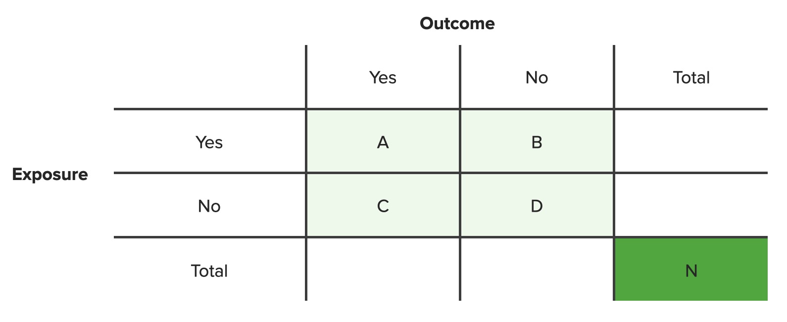
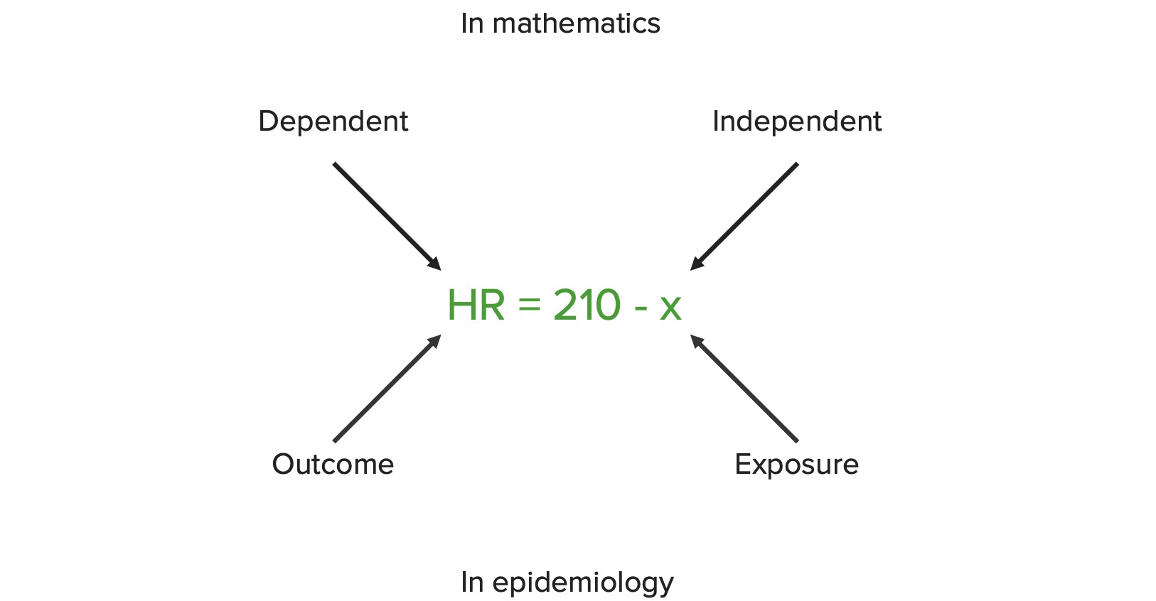
00:01 Welcome back to Lecture 2, where we're gonna discuss contingency tables. 00:06 So what is a contingency table? Well, it's a convenient way to display the distribution of two categorical variables together. 00:13 It's a table that provides information on how individuals are distributed along two variables, dependent on the value of the other. 00:21 We also call these things two-way tables and that can be used to obtain information about the distribution of each of the individual variables. 00:29 Here's an example, we're gonna look at educational attainment versus age group. 00:34 We have a sample of a 158,694 people and the educational attainment is down to left-hand side of the table. 00:43 The age group goes across the top and in each cell we have the number of individuals in our sample that fit into each pair of categories. 00:52 The number of individuals who are age 65 or older that did not finish high school, we see as 12,702. 00:59 Of the number of people who are 25 to 34 and finished four or more years of college is 10,168, and in total we have 158,691 individual sample. 01:13 What can we do with it? What’s the meaning of the counts and the percentages for each cell? Well, let's look at a couple of examples, what percentage of the sample contains -- consist of senior citizens who did not finish high school? What we saw that of the people that we surveyed 12,702 of them were senior citizens who didn't finish high school so this means that 8% of our sample consist of senior citizens that did not finish high school. 01:39 Let's look at another one. 01:42 What percentage of our sample is made up of persons age 25 to 34 who have four or more years of college? What we saw when we looked at the table that 10,168 people in our sample finish four or more years of college and were age 24 to 34, so that comprises 6.41% of our sample. 02:02 What other information is available from a contingency table? Well, we have these things called marginal distributions. 02:09 What we can get -- what that means is, we can get from the table of what the distribution of one of the two variable looks like all by itself without any relationship to the other. 02:21 The distribution of one of the variable by itself is known as that variable's marginal distribution and the variable corresponding to the columns of the table has its marginal distribution obtain by summing up the rows in that column for each of the columns in the table. 02:39 The marginal distribution of the column variable is obtained by looking at the column totals of the table. 02:46 Similar reasoning applies in obtaining the marginal distribution of the row variable. 02:53 For each row the marginal frequency of the category corresponding to the row can be obtained by adding up all the entries in that row. 03:02 And then we can look at the row totals to get the marginal distribution of the variable that goes down the left-hand side of the table. 03:09 Here's an easy way to remember what marginal distributions are, the marginal frequencies are given in the margins of the table. 03:18 The right margin gives the marginal distribution of the variable that corresponds to the rows, and the bottom margin gives the marginal distribution of the variable that corresponds to the columns. 03:29 So let's look at an example. 03:31 The first we're gonna look at the marginal distribution of educational attainment. 03:36 This first group is the marginal frequency of the number of people who didn't finish high school, and so we add up all the entries in the row for people who didn't finish high school and we get a total of 34,251. 03:52 So that means that 21.58% of our sample did not finish high school. 03:59 Now, we look at the group that finished high school, we add up all the entries in the row corresponding to finished high school and we get 61,259. 04:11 What that tells us is that 38.6% of our sample completed high school. 04:16 For the group that completed 1 to 3 years of college we just add up again all the entries in the row that corresponds to the 1 to 3 years of college and we get 29,165 people in our sample that finish 1 to 3 years of college for a percentage of 18.38%. 04:36 Finally, for 4 or more years of college, we add up all the entries in that row we got 34,019 people in our sample who finish 4 or more years in college and that gives a percentage of 21.44% of our sample completing at least 4 years of college. 04:53 We have to check our work once we're done finding the marginal distributions. 04:59 There's two things that we need to have satisfied, the first is that the frequency of each level of education should be equal to the total of the rows, and the second is that the relative frequencies should add up to 100%. 05:15 So let's check it out. 05:16 Okay, so are these two conditions satisfied? Well, the first one, yes. 05:23 If we look at the row totals in the table the frequencies that we came up with are in fact equal to those row totals, so that first condition is satisfied. 05:32 Secondly, we add up all the relative frequencies and they do add up to 100% so the works passes in two checks and we have found the marginal distribution of educational attainment. 05:43 Let's try another one. 05:46 Let's look at the marginal distribution of the age group. 05:49 We do a similar thing to what we did in education but now since the age group goes across the top the marginal frequencies are given by the totals of the columns corresponding to each age group. 06:01 So for the 25 to 34 age group, we add up all the entries in the 25 to 34 column and we get 42,905. 06:09 So that tells us that 27.05% of our sample is between the ages of 25 and 34. 06:16 For the 35 to 44 age group, we do a similar thing we get 38,663 in that column and so we have 24.36% in the age group 35 to 44. 06:32 Again, for the 45 to 54 age group, we add up all the entries in the column get 25,686 and so 16.18% of our sample is comprised of people between ages 45 and 54. 06:48 For the 55 to 64 age group, same thing we get 21,345 and so 13.45% of our sample is between ages 55 and 64. 07:02 Finally, for the over 65 group, we get 30,092 people and so 18.96% of our sample is at least 65 years old. 07:13 We gotta check our work again, since we found a different marginal distribution. 07:17 All of the frequencies in the age group add up to the totals in the bottom most row of the table so that first condition works out. 07:25 We add up the relative frequencies that we found in each column. 07:30 They do add up to a 100% and so our work checks out. 07:34 So we found the marginal distribution of the educational attainment before and we just now found the marginal distribution of the age group. 07:43 Other information that can be glean from the contingency table is the conditional distribution of one variable given the value of another. 07:52 Often we're interested in what the distribution of one variable looks like just for one value of the other. 07:59 For example, we might be interested in the distribution of educational attainment among the 45 to 54 year old age group. 08:07 Here, we only pay attention to the observations that fall in the 45 to 54 year-old age group, and here we'll only talk about relative frequencies. 08:17 We're gonna do this by example. 08:20 Let's go back to the educational attainment by age group example, and we're gonna look strictly at the 45 to 54-year-old age group. 08:28 The only observations that we're looking at are in the 45 to 54 age group, it’s as though the ones in the other age groups don't exist. 08:38 All percentages, all relative frequencies for educational attainment are computed now as a percentage of the people in the 45 to 54 age group and not as the percentage of the total sample. 08:49 Let's see how it's done. 08:52 Well, we have 25,686 people in the 45 to 54 age group so since this is what we're restricting our attention to. 09:01 This is the only group that we need to be concerned about so it's as though our entire sample right now is 25,686. 09:09 In that 45 to 54 age group we have 4,829 that did not complete high school so that mean 18.80% of the people in the 45 to 54 age group did not complete high school. 09:24 We have 10,300 in the 45 to 54 age group that did complete high school so that means that 40.1% of our 45 to 54 age group completed high school. 09:38 We have 4,598 who completed 1 to 3 years of college so 17.9% of the people in the 45 to 54 age group completed 1 to 3 years of college. 09:52 And finally, we have 5,559 people in the 45 to 54 age group who completed at least 4 years of college, and so 23.2% of the people age 45 to 54 completed at least 4 years of college. 10:09 Now, we have to check our work for the conditional distribution, to make sure that our distribution make sense. 10:16 We use the similar process to what we use for marginal distributions, we can complete a check on our work by making sure that the percentages that we came up with for the conditional distribution add up to 100%. So let's check it out. 10:30 We have 18.8 plus 40.1 plus 17.9 plus 23.2, which adds up to a 100%, so this indicates that our work was done correctly. 10:40 In other words, we have what would be a sensible conditional distribution. 10:45 What we've done now is we found the conditional distribution of educational attainment in the 45 to 54 year old age group. 10:53 All right, one question that we're often interested in is whether or not there’s actually a relationship between two categorical variables, in other words does knowing the value of one variable give us any information about the value of the other? And we call this, if the value -- if knowing the value of one variable doesn’t give us any information about the other, then, we'd say that these two variables are independent. 11:18 What do we mean by independence? When we say that two categorical variables are independent if the conditional distribution of one variable is the same for all categories of the other. 11:30 In other words, knowing the value of the other variable doesn't change the distribution of the first variable. 11:37 The easiest way to determine independence is to look at the conditional distribution of one variable for each category of the other. 11:45 Our first question is, are educational attainment and age group independent? In order to answer this question, we're gonna look at the conditional distribution of educational attainment for the 25 to 34 age group and see if it matches the one that we just found for the 45 to 54 age group. 12:04 Well, we'll go through and find the conditional distribution for the 25 to 34 age group, we have 42,905 people in the 25 to 34 age group, 13.9% of them did not complete high school. 12:18 40.8% of the 25 to 34 age group completed high school. 12:26 21.6% of the 25 to 34 age group completed 1 to 3 years of college and 23.7% of the 25 to 34 age group completed at least 4 years of college. 12:40 Now, we compare this to the percentages for the 45 to 54 age group. 12:45 In that age group we got 18.8, 40.1, 17.9 and 23.2%, these don't match. 12:54 We can conclude then that educational attainment and age group are not independent because the conditional distributions for, of educational attainment given the value of, or given the age group is not the same among the age groups. 13:13 All right, so determining independence in general, it's a lot easier to verify that two categorical variables are not independent than it is to verify that they are and the reason is that if two categorical variables are not independent we only need to show that two of the conditional distribution aren't -- don't match. 13:33 But if they are, we need to show this by finding the conditional distribution of 1 variable given each category of the other and show that all of them are the same and so it takes a lot more work to show that two variables are independent than it does to show that they're not. 13:50 One strange phenomenon that often happens when we look at contingency tables is known as Simpson’s paradox and simply stated what happens with Simpson’s paradox is that sometimes when we average across different values we can get really different results. 14:05 Let's look at an example and then we'll explain how Simpson’s paradox comes in to play. 14:10 Suppose Jack and Jill are pilots, and they're arguing about who’s the better pilot. 14:14 Jack argues that he's the better pilot because he landed 83% of his last 120 flights on time while Jill only landed 78%. 14:24 But if we examine the data more closely, what happens? We wanna look at day and night landings and see what we find. 14:31 So if we look at Jack during his day landings, he lands 90 out of 100 or 90% on time while Jill lands 19 out of 20 or 95% on time. 14:43 For day landings the percentages say that Jill is the better pilot. 14:48 What about night? Well, Jack lands 10 out of 20 or 50% of his night flights on time while Jill lands 75%, so she's also better at night, but overall Jack lands 83% of his flights on time and Jill lands 78% of her flights on time. 15:10 So what happens? Well, if we look at the day and the night percentages individually and they gave a different result in looking at the overall percentages, and why did this happen? Well, the reason is that the contribution to Jill’s overall on time rate is mostly for night flights, which has a lower success rate for both pilots. 15:30 Jack's landing are mostly done during the day, so while Jack has a better overall on time landing percentage, Jill has the higher percentage of on time landing in both day and night. 15:42 When this happens we have an example of what's called Simpson’s paradox. 15:46 This Simpson’s paradox happens when the conditional distribution within each value of the other variable show different results than the overall relative frequencies. 15:58 What's the big picture here? It's better to compare percentages within each level of the other variable because overall percentages can sometimes be misleading. 16:09 All right, so what can go wrong? What kind of mistakes can we make when we look at contingency tables? Well, there are several things that can happen. So here's a few things to watch out for. 16:19 First of all, we wanna make sure that the percentages for all marginal and conditional distributions add up to a 100%. 16:26 One thing that we don't wanna do is we don’t wanna confused similar sounding percentages. 16:31 Here's an example of two percentages that sound pretty similar. 16:35 The percentage of people who completed high school and are between 45 and 54 years old and the percentage of people who are between 45 and 54 years old that completed high school. 16:47 This sound very similar, but they're not the same thing. 16:51 The percentage of people who completed high school and/or between 45 and 54 years old that's one of the relative frequencies inside one of the cells in the body of the table. 17:03 However, the percentage of people who are between 45 and 54 years old that completed high school is a percentage that refers to a restriction to the 45 to 54 age group and the percentage within that group that completed high school. 17:19 We always wanna look at the variable separately as well as together. 17:23 We wanna be aware of Simpson’s paradox and we wanna make sure that we use a large enough sample size. 17:28 These are all examples of the most commons things that could go wrong in the analysis of contingency tables. 17:33 Remember these things when you look at contingency tables and when you’re finding marginal and conditional distributions and make sure that you're interpreting contingency tables appropriately. 17:45 All right, so that does it for Lecture 2, and we'll see you back here for Lecture 3 next time.
About the Lecture
The lecture Contingency Tables by David Spade, PhD is from the course Statistics Part 1. It contains the following chapters:
- Contingency Tables
- Marginal Distributions
- Checking the Work
- Conditional Distributions
- Independence of Two Categorical Variables
- Simpson's Paradox
Included Quiz Questions
What is a contingency table?
- A contingency table describes the distribution of two categorical variables at the same time.
- A contingency table describes the distribution of a categorical variable.
- A contingency table describes the distribution of two quantitative variables at the same time.
- A contingency table describes the distribution of a categorical variable over time.
- A contingency table describes the distribution of a quantitative variable over time.
What statement below is correct about marginal distributions?
- The marginal distribution of the column variable can be obtained by looking at the column totals of the table.
- The marginal distribution of the row variable can be obtained by looking at the column totals of the table.
- The marginal distribution of the column variable can be obtained by looking at the row totals of the table.
- The table shows only what the distribution of one of the two variables looks like.
- The table shows only what the distribution of one of the three variables looks like.
What is correct about conditional distribution?
- We only talk about relative frequencies.
- We only talk about absolute frequencies.
- Here, we only pay attention to the observations that take the given value of the first variable.
- Here, we cannot complete a check on our work by making sure that the percentages we came up with add up to 100%.
- We consider the importance of both relative and absolute frequencies.
Which of the following statements is correct?
- Two categorical variables are independent if the conditional distribution of one variable is the same for all categories of the other variable.
- Two categorical variables are dependent if the conditional distribution of one variable is the same for all categories of the other variable.
- If two variables are dependent, we need to show that all of the conditional distributions are different.
- The easiest way to determine dependence is to look at the conditional distribution of one variable for each category of the other variables.
- If two variables are dependent, we need to show that all of the conditional distributions are opposite.
What is Simpson’s Paradox?
- Simpson’s Paradox describes a situation when a trend appears for one group of data but disappears when groups of data are combined.
- Simpson’s Paradox occurs when the data comes out in a way that you do not expect.
- Simpson’s Paradox occurs when the marginal distributions of each of the two variables differ.
- Simpson’s Paradox occurs when the conditional distribution of one variable given one value of the other differs from the conditional variable of one variable given another value of the second variable.
- Simpson’s Paradox describes a trend that only appears when data are combined.
What is another term for a contingency table?
- Two-way table
- Two-times table
- Two-cross table
- Two-fold table
- Three-way table
What is true about the marginal frequency of the category corresponding to the row?
- It can be obtained by adding up all of the entries in that row.
- It can be obtained by multiplying all of the entries in that row.
- It can be obtained by dividing all of the entries in that row.
- It can be obtained by squaring all of the entries in that row.
- It can be obtained by adding all of the entries in other rows.
Relative frequencies should add up to which of the following?
- 100%
- 70%
- 80%
- 90%
- 0%
Percentages we come up with for conditional distributions must add up to which of the following?
- 100%
- 70%
- 80%
- 90%
- 0%
How may Simpson's Paradox be present in a contingency table?
- Simpson's Paradox may occur when the conditional relative frequencies within each variable differ from the overall results.
- Simpson's Paradox may occur when the marginal relative frequencies within each variable differ from the overall results.
- Simpson's Paradox may occur when the conditional relative frequencies within each variable are the same as the overall results.
- Simpson's Paradox may occur when the absolute frequencies within each variable differ from the overall results.
- Simpson's Paradox may occur when the absolute frequencies within each variable are the same as the overall results.
Author of lecture Contingency Tables

David Spade, PhD
Customer reviews
5,0 of 5 stars
| 5 Stars |
|
2 |
| 4 Stars |
|
0 |
| 3 Stars |
|
0 |
| 2 Stars |
|
0 |
| 1 Star |
|
0 |
It is better than that I watched in other web site. I really recommend this lecture.
Clear explanations that makes understanding of concepts easy. Relevant examples too
