Playlist
Show Playlist
Hide Playlist
Dosage Calculation: Maintenance Dose and Loading Dose – Elimination Kinetics

-
Slides Dosage Calculation Maintenance Dose Loading Dose.pdf
-
Reference List Pharmacology.pdf
-
Download Lecture Overview
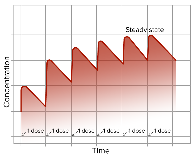
00:01 Let's talk about the concept of maintenance and loading doses. Let's use an example of drug X. 00:06 Drug X is a drug that requires very close monitoring of therapeutic levels. Here's a patient who takes 1 mg of drug X. Clearly 1 mg is not going to cut it for this patient, so we need to give him more everyday. 00:19 If he takes 1 mg every single day for 9 days, eventually we will get to the effective concentration that we want. 00:27 But that seems like a long time. Why don't we give him a whole bunch of medication at first, or what we call a loading dose? So here's an example of a patient who took 10 mg on day 1, you can see the concentration really climbs, and then after that we give him 1 mg a day. 00:43 That's the concept of a loading dose. So, for some drugs, we use loading doses all the time. 00:51 The loading dose can be calculated. It is a formula using bioavailablity, the target concentration, and the volume of distribution. So, it's Vd times the concentration divided by the bioavailability. 01:06 The formula is Vd equals the amount of the drug in the body divided by C. 01:10 Here, 'C' stands for the concentration of the drug in the blood or plasma. 01:15 If the Volume of Distribution is low, around 42 liters or less (which corresponds approximately to the body's total water volume), it indicates that the drug predominantly remains within the bloodstream or body fluids. This scenario is typical for drugs that are either too large to pass through cellular membranes easily or are heavily bound to plasma proteins, limiting their distribution into tissue spaces. 01:42 Conversely, a high Vd suggests that the drug extensively distributes beyond the blood and into the body's tissues. This is often seen in drugs with high lipid solubility. These substances can easily cross cell membranes and accumulate in fat tissues, significantly increasing their apparent volume of distribution. 02:04 Bioavailability refers to the proportion of a drug that enters the systemic circulation after being administered. This concept is crucial because not all of the administered dose reaches the bloodstream where it can exert its therapeutic effect. 02:19 We typically express bioavailability as a ratio of areas under the blood concentration-time curves. We compare the area under the curve (AUC) for a drug given via a route like oral (PO) to the AUC for the drug given intravenously (IV). 02:36 Since IV administration delivers the drug directly into the bloodstream, its bioavailability is considered 100%. 02:43 When a drug is taken orally, its bioavailability is often less than 100% due to: Incomplete absorption through the gut wall OR First-pass metabolism by the liver, where the drug is partially broken down before reaching systemic circulation. 02:58 In the image, which is used to illustrate the concept of bioavailability, you will notice two distinct curves: the IV curve is depicted in red, and the oral curve is in blue. The red IV curve typically rises quickly and directly to its peak because the drug is administered directly into the bloodstream, representing 100% bioavailability. This immediate peak reflects the direct and complete entry of the drug into the systemic circulation. 03:28 The blue oral curve, on the other hand, rises more slowly and to a lower peak compared to the red curve. 03:36 This difference is due to the drug’s passage through the digestive system and liver before it reaches the systemic circulation, leading to delays and reductions in absorption and, consequently, a lower bioavailability. 03:51 Now, the dosing rate, or how often we give the medication, is the clearance times the desired plasma concentration, once again divided by bioavailablity. Let's use bioavailability and volume of distribution to calculate dosing. Here is a case study of a 15 year old woman who has pneumonia. 04:12 She requires an antibiotic called supercillin, which of course doesn't exist. 04:17 It has a volume of distribution of 31 litres, and has an oral bioavailabity of about 55 %. 04:24 The required plasma concentration is 55 mcg/ml. What is the loading dose? Well, let's do the calculations together. We know that the loading dose is the volume of distribution multiplied by the concentration, and divided by bioavailablity. Let's plug in the numbers. 04:44 So you can see here that there is 31 litres times 55 mcg/ml divided by 55 %. That's 31,000 ml, right? So we're going to convert that. It's multiplied by 55 mcg/ml, and the percentage number, we're going to substitude 55 % in the denominator with 100 over 55. The loading dose is therefore 31,000 times 55 times 100 divided by 55, and cancelling out the 55, and cancelling out the millilitres, you get 3,100,000 micrograms or 3.1 grams. This 15 year old girl with pneumonia is getting worse. 05:29 The supercillin will be needed to be given intravenously. Supercillin, Vd of 31 litres, bioavailability 55 %, intravenous bioavailability of 99 %, and a required plasma concentration of 55 mcg/ml. The clearance is 6ml/min. 05:52 What's the dosing regimen of the drug? The dosing rate is the clearance times the concentration divided by bioavailability. The dosing rate is 6 ml/min times 55 mcg/ml divided by 99 %. 06:10 We do the substitution, we cancel out the millilitres, and we get 333 mcg/min, and if we multiply that into hours, we get 20 mg/hour. 06:27 Let's do a study on loading and maintenance dosing. A 66 year old woman had a cardiac arrhythmia which responded to lidocaine. The ideal serum concentration is 3 mcg/ml. The volume of distribution is 75 litres. 06:42 The clearance is 600 ml/min and the half life is 1.5 hours. The bioavailability is 100%. 06:52 What's the loading dose? And what's the ideal infusion rate? Okay. So, loading dose, once again, 75 litres is the volume of distribution. The target concentration is 3. 07:03 And the bioavailability is 100%. So we plug that into our equation, and we do the math, and we end up with 225 mg as your loading dose. The infusion rate is going to be your serum concentration multiplied by your clearance, divided by bioavailability. We are going to get an infusion rate of 3 mcg/ml times 600 ml/min times 100 over 100, which gives us 1800 mcg/min, or 1.8 mg/min.
About the Lecture
The lecture Dosage Calculation: Maintenance Dose and Loading Dose – Elimination Kinetics by Pravin Shukle, MD is from the course Pharmacokinetics and Pharmacodynamics. It contains the following chapters:
- Calculating Doses
- Case Study: Dosing
- Case Study: Dosing
Included Quiz Questions
The dosing rate is inversely proportional to what?
- Bioavailability
- Desired plasma concentration
- Clearance
- Volume of distribution
- Loading dose
The loading dose is proportional to which factor?
- Volume of distribution
- Half-life
- Clearance
- Bioavailability
- Age of the drug
Which statement regarding loading dose is most accurate?
- It is larger than the dose rate needed to maintain the concentration.
- It is a dose sufficient to produce a plasma concentration above the therapeutic window.
- It is a dose sufficient to produce a plasma concentration below the therapeutic window.
- It is smaller than the dose rate needed to maintain the concentration.
- The loading dose should never be administered to patients with a BMI < 20.
Author of lecture Dosage Calculation: Maintenance Dose and Loading Dose – Elimination Kinetics

Pravin Shukle, MD
Customer reviews
5,0 of 5 stars
| 5 Stars |
|
5 |
| 4 Stars |
|
0 |
| 3 Stars |
|
0 |
| 2 Stars |
|
0 |
| 1 Star |
|
0 |
