Playlist
Show Playlist
Hide Playlist
Distribution – Data

-
Slides 13 Data Epidemiology.pdf
-
Reference List Epidemiology and Biostatistics.pdf
-
Download Lecture Overview
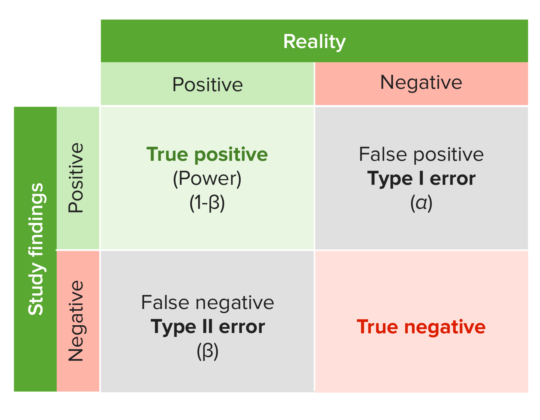
00:00 Okay, now let's say I have a sample of 10 students that are in my statistics class and their ages are 18, 18, 23, 25, 22, 25, 23, 18, 19 and 20. They're all very young, younger than me. 00:16 And I summarize the information that I had about their ages in a table. I've got three 18 year olds, one 19 year old, one 20 year old, one 22 year old, two 23 year olds and two 25 year olds, what can I do with that? Well I can depict that distribution of ages in something we call a frequency distribution. So from 18 to 20, I have four individuals, from 20 to 22, I've got one individual, from 22 to 24, I've got three individuals and from 24 to 26, I've got two more individuals. Depending upon how much I define the class differences in the widths that I care about, I can have a different shape of my frequency distribution. It is important though, because frequency distributions are used commonly in first understanding our data, but then to compute statistical tests on our data. What I'm getting at is something very special, that very special something is called the normal distribution. The normal distribution is a famous important special example of a frequency distribution. It has historical heft, many famous mathematicians lay claim to having discovered the normal distribution and it's called many things, the bell curve, the Gaussian distribution. 01:28 It doesn't matter. It's just a histogram that describes a distribution of many human characteristics. 01:35 What it says is, most things have a number of occurrences that are common and a number of occurrences that are less common, that's all it's really saying. But there is something magical about the normal distribution and here's how it works. It's called the central limit theorem. This is what the central limit theorem says. It says if I'm measuring something, let's say I'm measuring the average age of students at my university and I decide to take a sample of students, of 20 students and measure their average age as a sample and I get a certain number. I put those students back into the pool, I take another group of 10 students and I measure their age and compute the average. I put them back in the pool, I take another and so forth. I do this an infinite number of times. I'm going to get a different average each time, but there will be sometimes it repeats itself, sometimes I'll get one repeated many times. If I were to draw a distribution, a frequency distribution of the times that I get something, one or two of these I will get very, very frequently, a few others I'll get less frequency, but a magical thing happens, if I do it an infinite number of times, my frequency distribution when I collect a bunch of samples will look like this, like a normal distribution, that's called the central limit theorem. Essentially says that pretty much every characteristic, when sampled in this infinite fashion, eventually will describe a normal distribution. Why is this useful? Well it means that if I take a sample now and the mean of my sample is from one of the extreme parts of the curve, it may not be a typical example. It'll be unusual, because the usual ones are from the center of this curve, they're typical. How typical do I care about? Well that depends. 03:29 The more I get to the tails, the extremes, the more untypical I get, the more unusual I get. Now if I get a really unusual one, maybe this represents a whole different universe of truth. Now we're into the realm of statistical significance. So P-value is when our test result falls under this curve. A P-value tells me the probability of how likely my sample is from which part of the curve. If my p-value is from one of the extreme parts and it's less than a certain cutoff value, I can conclude that my sample is so unusual that I can probably reject the null hypothesis and say that my sample represents a whole different hypothesis, a whole different reality. The size of my rejection zone, where I'm going to find the cutoff of my p-value is called a type I error and that's a variable. I couldn't decide where I set that, but historically, we set it somewhere useful, we set it at about 0.05.
About the Lecture
The lecture Distribution – Data by Raywat Deonandan, PhD is from the course Data.
Included Quiz Questions
What is the significance of the p-value?
- It allows one to accept or reject the null hypothesis.
- It is a numerical representation of the mean of a data set.
- It is a representation of absolute risk reduction.
- It is a representation of relative risk reduction.
- It represents the true odds ratio.
What is the vertical axis (Y) used for in graphing frequency distributions?
- To display frequency
- To display categories
- To display scores
- To display population
- To show percentile
Author of lecture Distribution – Data

Raywat Deonandan, PhD
Customer reviews
5,0 of 5 stars
| 5 Stars |
|
5 |
| 4 Stars |
|
0 |
| 3 Stars |
|
0 |
| 2 Stars |
|
0 |
| 1 Star |
|
0 |
